Chapter 7 Simulation and modeling

profiler is R a tool that allows you to check the performance of your functions and would help you optimize

The str() function gives a quick examination of R objects functions and data properties, useful for having a general idea of what an specific expression is.

str(str)
library(datasets)
head(airquality)
str(airquality)
s <- split(airquality,airquality$Month)
str(s)

7.1 Simulation

because R is statistics orientated it has many functions used for creating distributions. Each type of distribution like normal, Poisson, etc. has associated the following prefixes that specify different outcomes.

d: density
__r:__random number generation
p: cumulative
q: quantile

The following are some examples.

rnorm: normal distribution given a mean and a standard deviation
dnorm: Probability density
pnorm: Cumulative distribution from a normal distribution

*rpois: generates a random Possion distribution given a defined rate

library(datasets)
with(airquality,tapply(Temp,Month,mean))

##        5        6        7        8        9 
## 65.54839 79.10000 83.90323 83.96774 76.90000

Temperature<- airquality$Temp

model <-rnorm(153,mean(Temperature),sd(Temperature))
 

plot(density(Temperature))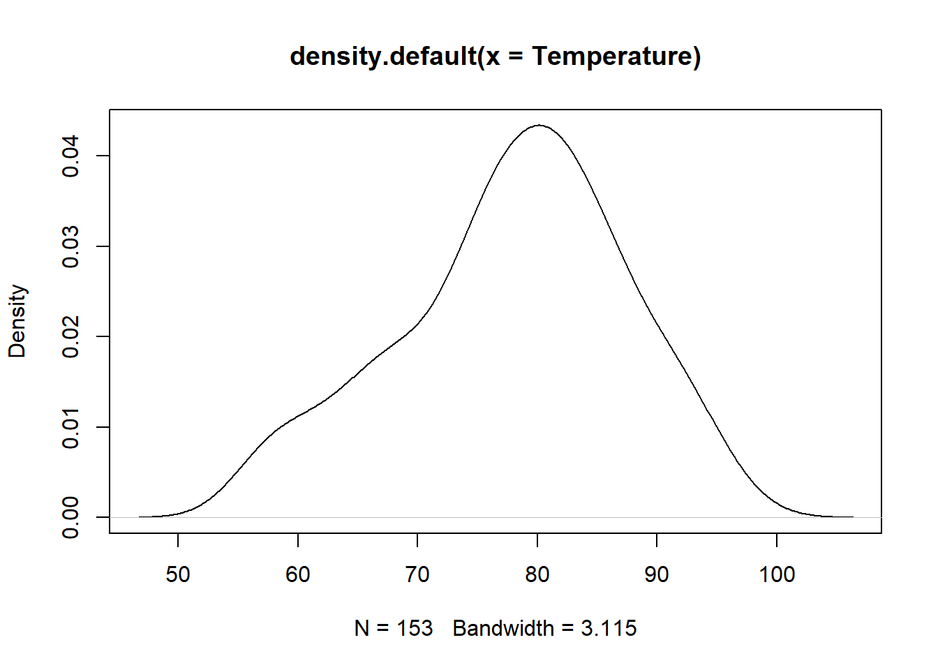

Figure 7.1: air density

plot(density(model))

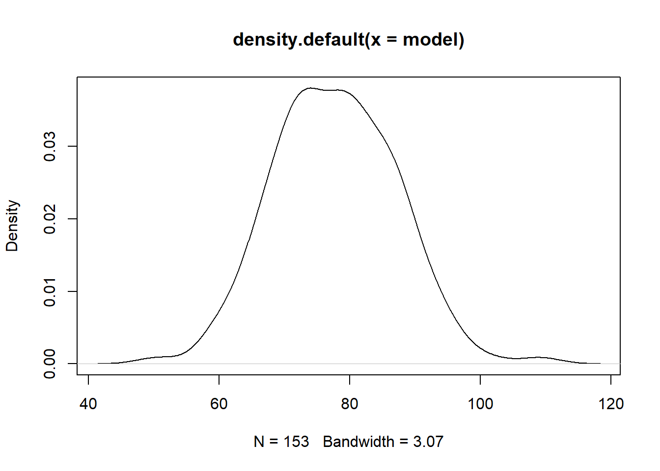
Figure 7.2: air density

R produces random number that are not entirely random, instead they are made through a pseudo random generator, an algorithm that will map the output to a list of values with a determined probabilistic distribution. A seed will determine the behavior of the algorithm, any seed will always map to the same numbers. It is important to be able to reproduce the exact same results, so the set.seed() function is used to ensure that the random values generated stay the same.

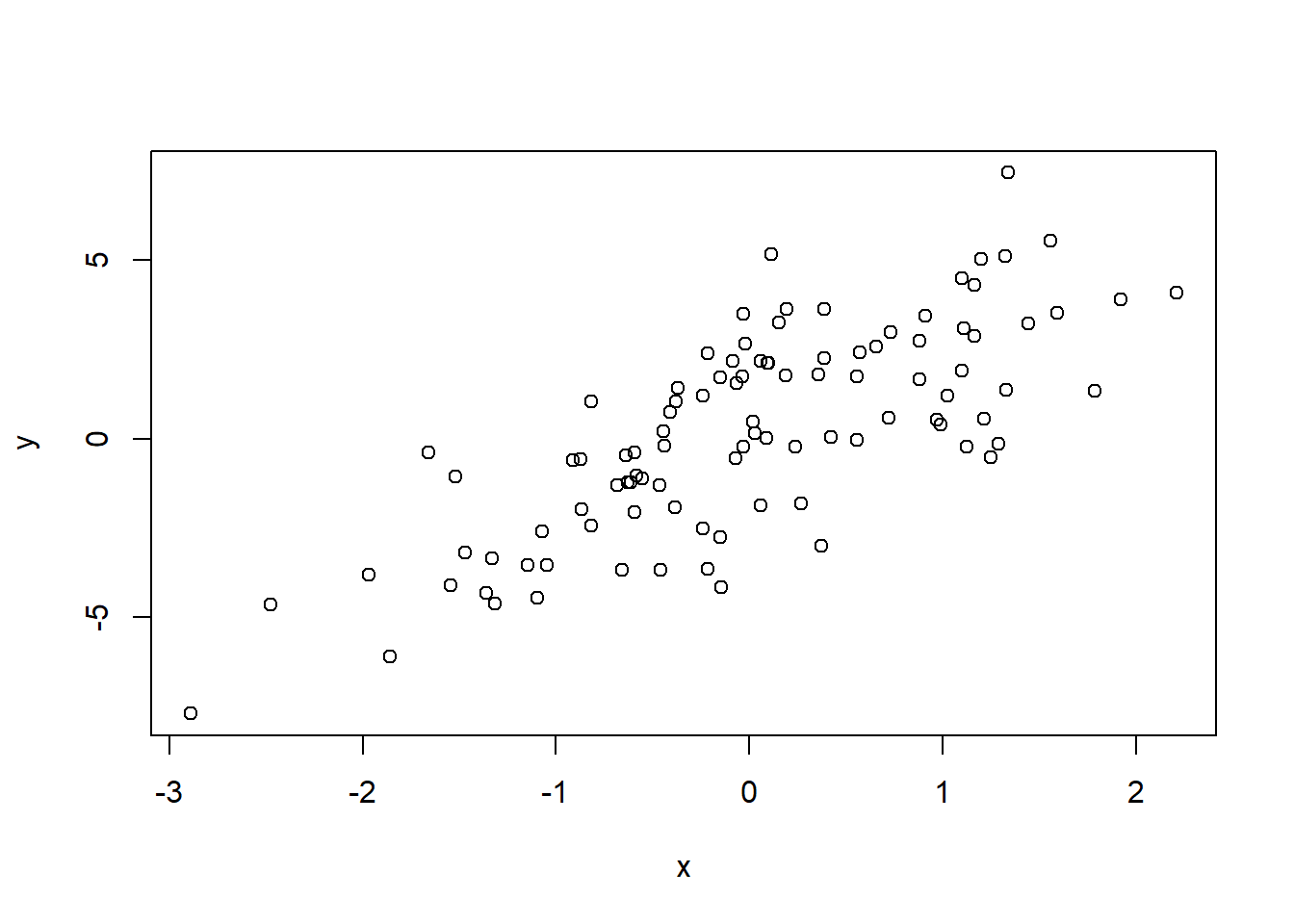
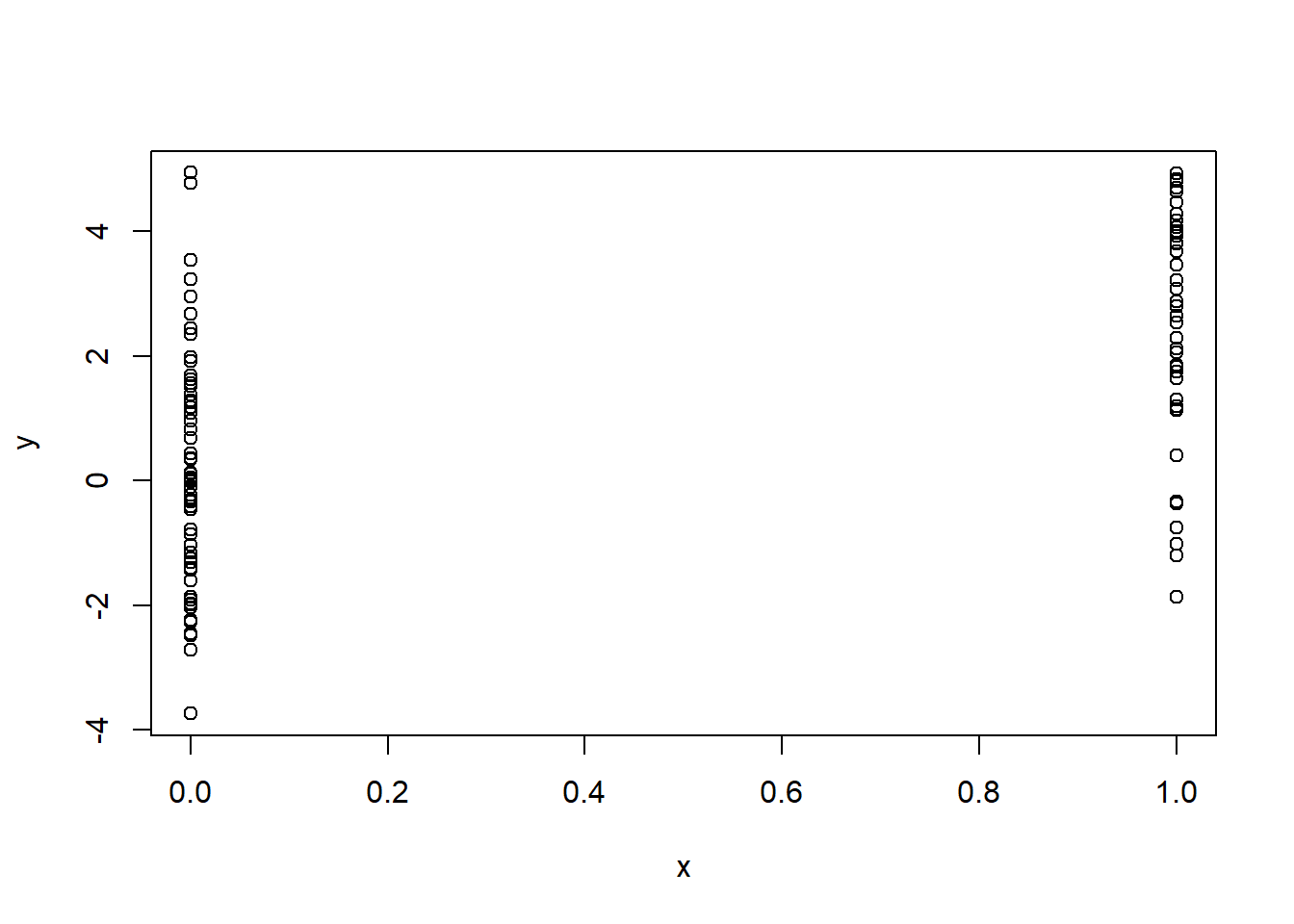
print(" set seed to 3")

## [1] " set seed to 3"

set.seed(3)
rnorm(5)

## [1] -0.9619334 -0.2925257  0.2587882 -1.1521319  0.1957828

print("seed not set ")

## [1] "seed not set "

rnorm(5)

## [1]  0.03012394  0.08541773  1.11661021 -1.21885742  1.26736872

print(" set seed to 3 again")

## [1] " set seed to 3 again"

set.seed(3)
rnorm(5)

## [1] -0.9619334 -0.2925257  0.2587882 -1.1521319  0.1957828

We want to create a linear model of the form

\[\begin{equation*} y= \beta _1 + \beta_2 x +\epsilon \tag{7.1} \end{equation*}\]

set.seed(20)
x<- rnorm(100)
set.seed(10)
e <- rnorm(100,0,2)
y<- 0.5 + 2*x + e
plot(x,y)

set.seed(10)
x<- rbinom(100,1,0.5)
set.seed(10)
e <- rnorm(100,0,2)
y<- 0.5 + 2*x + e
plot(x,y)

7.2 sampling

7.3 Code Optimization

R profiler examines how much does it take to run a piece of code

#Rprof("../data/Profile.out")
#source("../code/covid_19.R",echo=FALSE)
#Rprof(NULL)
details<-summaryRprof("../data/Profile.out")

## Warning in readLines(con, n = chunksize): incomplete final line found on '../
## data/Profile.out'

head(details$by.self)

##                         self.time self.pct total.time total.pct
## "charToDate"                 3.80    73.36       3.80     73.36
## "scan"                       0.96    18.53       0.96     18.53
## "as.Date"                    0.08     1.54       3.86     74.52
## "FUN"                        0.04     0.77       0.08      1.54
## "mget"                       0.04     0.77       0.04      0.77
## ".rs.getHelpFromObject"      0.02     0.39       0.24      4.63

The time spend be of tow different categories $by.self or by.total the latter has the disadvantages that it records the time full time the top level function tend to spend must of the time can What

by the example we can see that must of the time is spent on converting data into Date type. we

library(profvis)

7.4 SWIRL practices

As part of this weeks activities the following swirl practices

7.4.1 Looking at Data

when first introduce to a dataset you need to gain a broad understanding of the data, R has many functions usefull for exploratory analysis, pocking around the data and knowing what it is in there.

dim()
names()
object.size() allows you to know how much space a dataset is occupying in memory
summary() is very useful to get a sense of the data it give properties such as the mean, the median, the number of NA values, etc.
table()
str()

7.4.2 Simulation

simulate the probability of a flip of a coin with an skewed probability of 70% head and 30% tails. We could use sample with replacement and specify to find the number of times it would land heads making 100 flip, how ever the binomial distribution function rbinom to simulate the expected value, and not only once but the times necessary

set.seed(1)
rbinom(1,size=100,prob=0.7)

## [1] 68

set.seed(13)
heads<- rbinom(500,size=100,prob=0.7)

hist(heads)

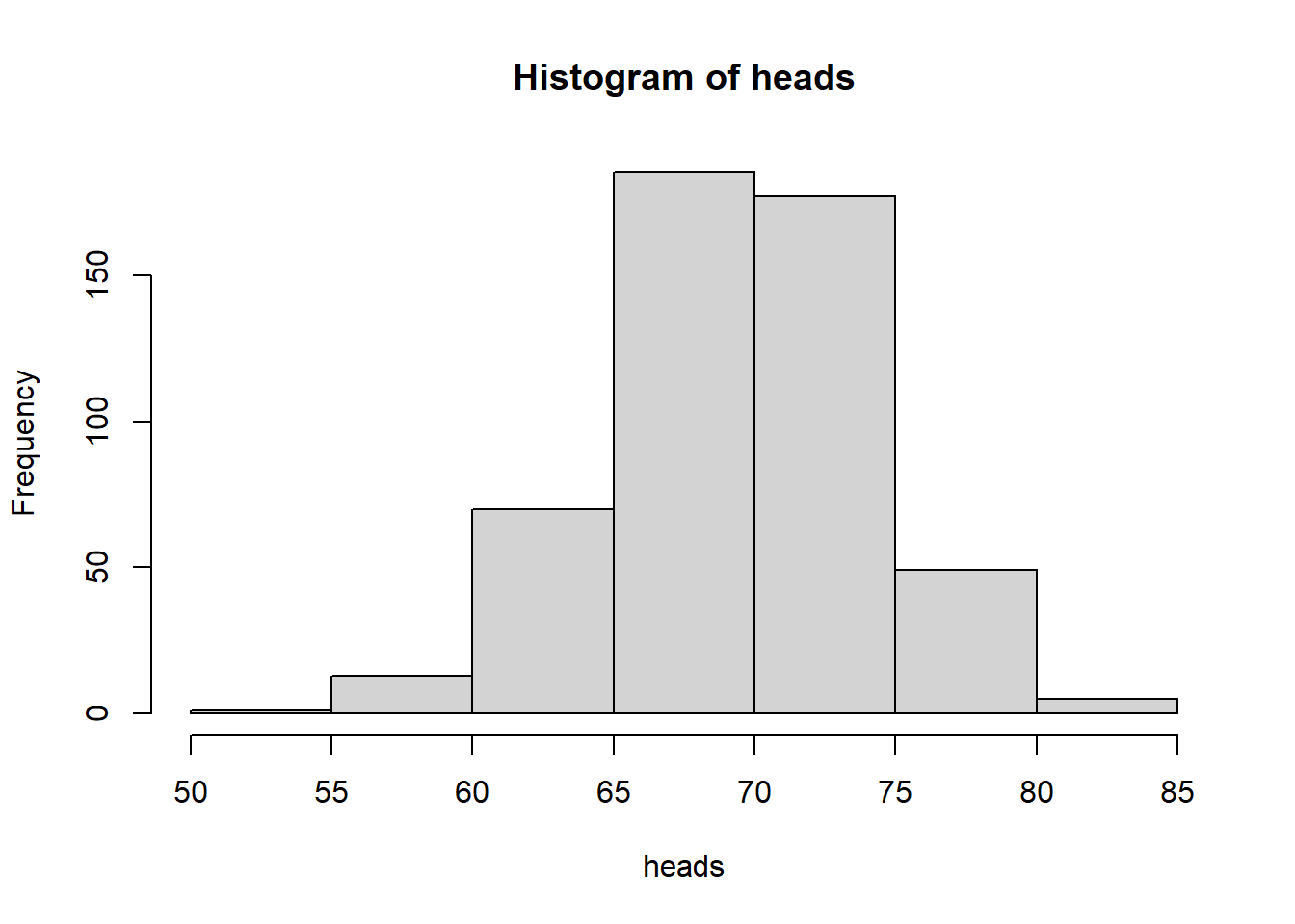
Figure 7.3: heads expected of 100 coin flips

range(heads)

## [1] 51 84

Generate 100 groups of random numbers each one of 5 vaules generate with a Poisson distribution with mean 10

set.seed(19)
rpois(5,lambda = 10)

## [1]  6  5  8 13  9

my_pois<- replicate(100,rpois(5,10))

Other distributions: exponential rexp(), chi-squared rchisq(), gamma rgamma()

7.4.3 Base Graphics

lattice, ggplot2 and ggvis

http://varianceexplained.org/r/teach_ggplot2_to_beginners/

http://www.ling.upenn.edu/~joseff/rstudy/week4.html

load data

plot is to scatterplot

“formula” interface plot(dist ~ speed, cars)

xlab = “xlabel”, ylab=“ylabel”, main =“title” sub=“My Plot Subtitle” col=2 color red ?points pch=2

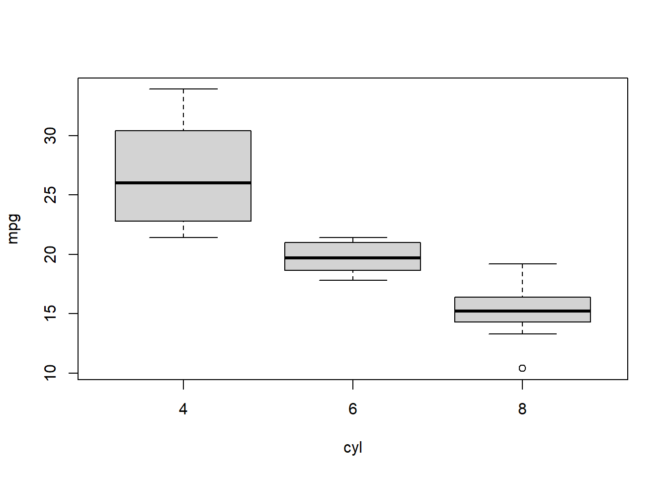
?boxplot

data(mtcars)
boxplot(mpg~ cyl, data=mtcars)

Data Science course notes